Training a 3.8B LLM to 0.384 CORE for $998
Somewhere between “nanoGPT toy” and “you need a research lab” there’s a large, under-described region where one person with a few thousand dollars can train a meaningful model.
I wanted to see language and understanding emerge from random weights for myself, and to learn the parts you can only learn by starting from scratch. This project was written in the evenings, debugged on a 5090 and finished on rented B200s. It was heavily inspired by Andrej Karpathy’s nanochat.
The result is a 3.8B-parameter model scoring 0.384 on CORE, trained on 65B tokens in 43 hours for $998.
What follows is what worked, what didn’t, and what I still don’t know.
| Model | Params | Tokens | Hardware | Time | Cost | CORE |
|---|---|---|---|---|---|---|
| GPT-2 (OpenAI) | 1.5B | — | — | — | — | 0.2565 |
| nanochat d26 | ~561M | 11.2B | 8× H100 | ~3h | — | ~0.258 |
| nanochat d32 | ~1B | — | 8× H100 | ~33h | ~$1000 | 0.310 |
| little-lm 3.8B (1024 ctx) | 3.848B | 57.3B | 8× B200 | 35.9h | $820 | 0.338 |
| little-lm 3.8B (2048 ctx) | 3.848B | 65.3B | 8× B200 | 43h | $998 | 0.384 |
My model is larger than nanochat d32 and took similar wall-clock time. B200s were better value per unit of work than H100s. But for roughly the same money as nanochat’s $1,000 configuration, this lands meaningfully ahead of it. An encouraging data point about what’s reachable outside a lab or a mega company with millions in compute budget. As the frontier moves, $1,000 takes you further and further.
Setup
I’ve built little-lm as a config-driven framework for training small decoder-only LLMs. Every run is fully specified by a YAML file: model, dataset, optimizer, schedule, callbacks. Components self-register into a global registry and get resolved by name, so swapping an optimizer or a dataset is a one-line config change.
Good infrastructure pays for itself almost immediately. Ordinary software engineering discipline (Things like separation of concerns, clean interfaces, components you can swap in) matters a lot in AI work. It cost me a little at the start, and a couple more times afterward to fix bad contracts or suboptimalities. But this time investment pays for itself at the first convergence problem you encounter. I found that a great infra is the infra that almost never requires you to edit code manually. If you can read the config and understand exactly what happens, and there are no hidden mechanics, it means you have done a good job. The following report is the result of being able to express experiments as a three-line YAML diff rather than a branch.
The final model is Llama-style: RMSNorm, RoPE, GQA (24 query heads, 8 KV heads), relu² MLPs, QK-norm, logit softcap, per-layer learnable residual scalars, and ResFormer-style value embeddings.
| Component | Params |
|---|---|
| Token embeddings | 154.5M |
| LM head (untied) | 154.5M |
| 28 decoder layers | 2,818.7M |
| Value embeddings (14 tables) | 721.2M |
| Total | 3.848B |
Worth noting that the value embeddings are 19% of the parameter count. 14 tables of vocab × kv_dim, one on every other layer.
Results
Early experiments
Before good runs there were many bad ones.
I trained an 858M Llama on FineWeb-Edu for 16.4B tokens, 5.8 days on a single A100. AdamW at 2.5e-4, cosine decay to zero, 5% warmup, batch 256 via gradient accumulation, 2048 context.
The result: PIQA 60.45%. GPT-2 124M scores about 63%. I had spent six days of compute to build something worse than a model seven times smaller, from 2019. Generations were repetitive and borderline nonsensical.
The loss curve told the story.
- Cosine decay to zero. The curve went completely flat after about 70% of the steps. The final 30% of the compute budget produced essentially nothing as the learning rate might be too low. Linear cooldown holds a useful rate much later.
- Peak LR too conservative. 2.5e-4 is low for 858M parameters. You can be quite aggressive for those small models.
- AdamW on everything. Muon should be meaningfully better per-token for the matrix parameters at this scale. In fact this was demonstrated pretty quickly in ablation runs.
- The data. FineWeb-Edu is decent. It is not the best available.
Five changes came out of that post-mortem. Together they are the difference between the run above and a model that beats GPT-2 by a wide margin.
Trapezoidal LR schedule. Warmup for 5%. Hold flat and finish with linear cooldown over the last 50% to 5% of peak. The point is that the model keeps learning until the end instead of coasting through the tail. In the 3.8B run the eval loss was still descending at the final step, which is exactly the behavior the 858M run failed to produce.
Muon for matrix parameters, AdamW for everything else. Muon is slower per step (Newton-Schulz orthogonalization isn’t free, about 25% in a shallow-accumulation benchmark) but that cost is paid once per optimizer step: at 7 gradient-accumulation steps it dilutes to ~4%. Measured against total run time the convergence is much faster overall.
ClimbMix instead of FineWeb-Edu. This was a tremendous jump in convergence speed. Exactly as Karpathy found as well.
FP8 + vocab padding. FP8 training via torch._scaled_mm with dynamic tensorwise scaling on all three GEMMs, and padding the vocab from 50,257 to 50,304 (a multiple of 64) so the tensor cores are happy. Together, +33% throughput mostly from fp8.
1024 context instead of 2048. Halving the context roughly doubles the batch size at fixed memory. Throughput barely changes per token. We are still dominated by the MLPs which is a good sign we are using the hardware effectively. Below we will discuss the impact of the context length on the model.
Here is the whole run:
| Step | Tokens | Eval loss | CORE |
|---|---|---|---|
| 2,500 | 5.7B | 2.3278 | 0.2389 |
| 5,000 | 11.5B | 2.2072 | 0.2752 |
| 7,500 | 17.2B | 2.1571 | 0.2934 |
| 10,000 | 22.9B | 2.1269 | 0.3104 |
| 12,500 | 28.7B | 2.1075 | 0.3147 |
| 15,000 | 34.4B | 2.0710 | 0.3224 |
| 17,500 | 40.1B | 2.0395 | 0.3294 |
| 20,000 | 45.9B | 2.0160 | 0.3267 |
| 22,500 | 51.6B | 1.9963 | 0.3345 |
| 25,000 | 57.3B | 1.9868 | 0.3384 |
~480,000 tokens/sec in steady state, which puts 57.3B tokens at 33 hours. The wall clock was 35.9h. The difference is the CORE evaluations, which took about 15 minutes each (ten of them over the run) and consumed 7% of the total.
Re-running this identical recipe at 2048-token context scored 0.3840. Almost all of that gap turned out to be some tasks that were very context dependent.
On the GPUs themselves: 92% SM activity, 40% SM occupancy. High activity means the SMs almost never went idle. No dataloader starvation or network waits, which is the payoff for downloading the shards locally instead of streaming, which would leave us vulnerable to a small hugging face network hang. The low occupancy is what back-to-back large GEMMs look like: matmul kernels trade occupancy for register-tile size on purpose. Compute-bound and well fed, great signal we are using the hardware well and we can extend every dollar we spend into a better model.
That’s about 1,047 TFLOP/s sustained per B200, or ~25% MFU against Blackwell’s dense FP8 peak. (Against the bf16 peak it reads as 50%, which is the number that matters a bit more because not even all the linear layers run in FP8.)
The distributed strategy is plain old DistributedDataParallel. At 3.8B on a single node, gradient communication was never the constraint, and the sharded-optimizer machinery turned out to be unnecessary.
Increasing throughput
Renting GPUs isn’t cheap, at work you often think about the quality of the model before its cost. When it’s your own money burning, throughput matters a lot more all of a sudden.
This took real work on a single RTX 5090, before I ever rented a node. Baseline 858M model, bf16, compiled: 26,144 tok/s. Final: 37,621 tok/s.
FP8 (+25%). All three GEMMs (1 forward and 2 backwards) in FP8 with dynamic tensorwise scaling. Requires SM90+ but that is quite a nice throughput jump.
Vocab padding (+33% cumulative). Padding 50,257 → 50,304 costs 47 unused embedding rows and unlocks the fast tensor-core path. Nearly free.
Fused linear cross-entropy (+44% cumulative). Liger’s FusedLinearCrossEntropyLoss fuses the lm_head matmul into the loss and chunks internally, so the full (B*T, vocab) logits tensor is never materialized. Measured head-to-head at the same batch size it is 6% slower:
| Config | Throughput | VRAM |
|---|---|---|
| Baseline CE, batch 6 | 34,724 tok/s | 27,852 MiB |
| Fused CE, batch 6 | 32,952 tok/s | 19,630 MiB |
| Fused CE, batch 8 | 35,979 tok/s | 24,028 MiB |
| Fused CE, batch 10 | 37,621 tok/s | 28,872 MiB |
Even though it’s slower per step, it buys back a good amount of VRAM (8 GB on my 5090) so the increase in micro-batch size more than makes up for the lost 6%. Claude was quick to reject it because it was 6% lower, but overall it was a great way to claw some extra throughput.
Non-gated MLPs. Dropping the gate projection (SwiGLU → relu², two matmuls instead of three) on the small model: 183,035 → 214,173 tok/s and 6 GB less VRAM. One caveat from the ablations: a SwiGLU intermediate ratio of 2.75 does not transfer to relu². The model learns noticeably worse. Use 4× for non-gated.
bf16 master weights. Keeping the optimizer master weights in bf16 rather than fp32 cut VRAM 27% and raised throughput from 640K to 1.4M tok/s on the 1.5B config. That was a huge speed-up, 2.2×. The quality cost is real but small: CORE 0.22 vs 0.23 at 4,000 steps. When you’re optimizing for capability per dollar, careful dtype handling is one of the highest-leverage and underdiscussed knobs available.
Hardware. Same code, 150M model, FP8: RTX 5090 at 184,662 tok/s, B200 at 477,440 tok/s. 2.59× from hardware alone, before accounting for the extra VRAM letting you push batch size further.
What didn’t work
Document-boundary masking with flex attention. Packing documents into one sequence lets tokens attend across boundaries, so I fixed it properly: per-token document IDs and mask out attention so each token can only attend to its current document. It was elegant, but I deleted all of it. Andrej Karpathy also found that cross-document leakage does not make things much worse under BOS-aligned packing. Best-fit packing replaced it in ~10 lines, and attention went back to an unconditional F.scaled_dot_product_attention(..., is_causal=True). I believe this is also conditional on the dataset and the training documents.
Liger RMSNorm and RoPE. RoPE was 2.2× faster in a microbenchmark and produced no measurable change in end-to-end throughput. RoPE is not part of the critical compute bottleneck at this scale. RMSNorm was outright slower than PyTorch 2.9’s built-in F.rms_norm (0.41ms vs 0.25ms). Both reverted, not worth the complexity.
Nanochat-style initialization. Embeddings at N(0, 0.8), linear weights uniform, output projections zero-initialized so the residual stream starts as pure identity, LM head at N(0, 0.001). Theoretically much nicer than GPT-2’s N(0, 0.02) everywhere. The loss curve starts marginally lower and the two curves overlap by ~1,500 steps. No measurable quality difference. I kept it, but for aesthetics, not evidence.
Streaming datasets. Great for getting started, wrong for a real run. Even when the network looks healthy, local shards gave 2-3% more throughput, and occasional network dips cost far more than that. For runs longer than a few hours, it’s worth it to pay the download once at the start of training.
Ablation on value-embedding
Value embeddings were 721M parameters for a 3.8B model. I trained the same model with the same config with value_embeddings: false and compared it against the original run, which I’d already paid for, out to 12,500 steps and 29B tokens.
| Params | Loss @12.5K | CORE @12.5K | Throughput | |
|---|---|---|---|---|
| Value embeddings on | 3.848B | 2.1075 | 0.3147 | 479,445 tok/s |
| Value embeddings off | 3.128B | 2.1171 | 0.3047 | 477,908 tok/s |
0.46% better loss and 3.2% better CORE, for 19% more parameters. The throughput is identical, because value embeddings are lookups. They cost memory and optimizer state but essentially no FLOPs.
Two interesting findings:
- Value embeddings bought the equivalent of about 1,200 training steps. Here is how to price that: between steps 10,000 and 12,500 my baseline loss fell 0.0194, so 2,500 steps buys roughly that much. The value-embedding advantage is 0.0096, about half of it — call it 1,200 steps out of 25,000. So 19% more parameters is worth ~5% more training.
- CORE moved about seven times more than loss did (3.2% vs 0.46%), and the gap shrank steadily during training. That’s worth knowing if you’re using CORE to make decisions: it’s an accuracy metric, so items near the decision boundary flip on tiny logit changes, and it’s centered against a random baseline, which amplifies relative differences while scores are still low.
Value embeddings are useful for a small model and come at almost no throughput cost. Spending a little bit of VRAM on this gives the model a form of bias toward certain concepts that might be useful for CORE.
Discussion
Misleading micro-benchmarks
We could be tempted to believe that 1024 tokens context is plenty for a high CORE score. Going back through the per-task logs, that conclusion is wrong on some tasks that are very context sensitive.
3 of the 22 CORE tasks have prompts that essentially never fit in 1024 tokens:
| Task | Prompts cropped | Step 2.5K | Step 25K |
|---|---|---|---|
| squad | 10570 / 10570 (100%) | 0.1478 | 0.0000 |
| boolq | 3265 / 3270 (99.8%) | 0.5798 | 0.5131 |
| bigbench_language_id | 9965 / 10000 (99.7%) | 0.2454 | 0.2538 |
SQuAD is the striking one. It doesn’t stagnate, it decays monotonically to exactly zero: 0.1478 → 0.0617 → 0.0099 → 0.0007 → 0.0000. The model gets steadily worse at this task the longer it trains, which is not a thing models normally do.
Two details explain it. SQuAD is a 10-shot task in the DCLM bundle, so each prompt is ten worked examples followed by the real one. Median of 1,998 tokens on my eval data. Not one fits in 1024. And when a prompt is too long my harness keeps the last max_seq_len tokens.
The test passage sits at the end, so it always survived; a test example is only ~169 tokens. What got truncated was the ten demonstrations. The model was reading the passage and the question, and almost never seeing the examples that teach it the expected output format. Since SQuAD is scored on exact-token match against the gold answer, fluent prose scores zero every time.
That also explains the decline. An early, high-entropy model occasionally emits something short and generic that happens to match. As it sharpens it commits to well-formed continuations, and the accidental hits disappear. Funnily enough, getting better at language made it worse at guessing right by accident.
boolq shows a gentler version of the same shape. It peaks at step 10,000 (0.6294) and declines to 0.5131. Language identification never moves off chance at all.
In short, 0.338 was measured with three of 22 tasks scoring near-zero for reasons that have nothing to do with model quality, just the size of the context length being fed to it.
The effect of larger context
As we have seen, if we want the highest CORE score possible we need larger context. But this has consequences on the training throughput.
Double the context length, halve micro-batch to hold VRAM constant, so tokens per optimizer step stayed identical. I stopped it at ~28,000 steps to save the last few hours of rental, so the learning-rate warmdown never fully completed and the number below is a lower bound.
CORE went from 0.3384 to 0.3840.
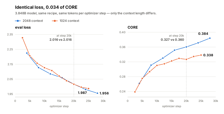
At step 20,000 the two runs have the same eval loss to four decimal places (2.0160 vs 2.0164) and differ by 0.034 on CORE. It was surprising to see that low level of correlation between CORE and eval loss on the ClimbMix dataset.
| Task | 1024 | 2048 | Cropped |
|---|---|---|---|
| squad | 0.0000 | 0.3114 | 100% → 47% |
| boolq | 0.5131 | 0.7095 | 99.8% → 3.2% |
| bigbench_language_id | 0.2538 | 0.2585 | 99.7% → 14% |
| the other 19 tasks | +0.008 combined |
squad and boolq alone are 83% of the gain. boolq contributes the most, because its random baseline is 0.5 and CORE centers against that: a raw +0.196 becomes a centered +0.517. Strip those two and the remaining twenty move +0.008 in total, roughly what 14% more tokens buys on its own.
Language identification went from 99.7% cropped to 14% cropped and moved +0.005. This is by far the hardest task in the CORE evaluation benchmark for our current model.
A couple of tasks got worse: commonsense_qa dropped 0.072, cs_algorithms 0.031. Across 22 tasks some movement in both directions is expected.
2048 was worth paying for as a measurement decision, not a quality one. It cost 9% throughput (480K → 437K tok/s), and outside the tasks that couldn’t be scored at 1024 it bought almost nothing. 1024 is fine for training and a “cheap” way of getting your model to a good CORE score. 2048 unlocks some tasks that are very context bound.
Future work
Limitations
Four things I never ablated. Peak LR, from nanochat’s sqrt(768/d_model). I didn’t really want to spend money to sweep learning rates. I moved from cosine to trapezoidal because of the 858M post-mortem, there could be schedules out there that are more efficient. QK-norm, on by default and never toggled off. And the GQA ratio, since it’s a nice lever to save on memory.
Most of those are inherited from nanochat rather than tested here. That is a defensible way to spend a small budget — someone else already paid for the experiment — but it means I am trusting that Karpathy’s results transfer to my model, data and scale.
Open questions
There is a lot of interesting work I’d want to pursue if I had more time and resources:
- Value embeddings versus reallocation. The comparison above was VE against nothing. The one that matters is VE against spending those 721M on something else.
- 1024 versus 2048 at matched wall-clock. The rerun changed context and ran longer, so it settles the measurement question but not the quality one.
- Why commonsense_qa regressed by 0.072 at the longer context, when nothing about that task involves long prompts.
- Sharding the optimizer, the way nanochat does. I used plain DDP with a single-GPU Muon, which means every rank holds a full copy of the optimizer state and redundantly recomputes the same Newton-Schulz update. nanochat drops the DDP wrapper entirely and does ZeRO-2 sharding inside the optimizer, overlapping reduce-scatter, compute and all-gather. The memory win is the certain one, and freed memory turns into batch size, which is tokens for the same dollars. Whether the redundant orthogonalization also goes away depends on how the sharding is done: Muon needs the full gradient matrix, so splitting a matrix across ranks doesn’t help, while giving each rank whole matrices of its own would. I haven’t explored that at all but I think it would be a great way to further increase the total training throughput at the cost of some extra machinery.
- Additional data exploration. I haven’t had a lot of time for data analysis on either the CORE benchmark or the ClimbMix dataset. I’m sure this would help us claw even higher performance with the same compute budget.
Closing thought
GPT-2 was a frontier result in 2019, produced by a well-funded lab with a large team, and its 1.5B model scores 0.2565 on CORE. 7 years later I beat that by a wide margin in my evenings, for $998, on hardware I rented by the hour.
The frontier moved, and everything came with it. Work that needed a lab can now be done by a single engineer in the evenings. I wonder what kind of insane machine we will be able to build in 7 years from now!
Appendix: the config
The whole run, flattened from the YAML includes into one block.
model:
  hidden_size: 3072
  intermediate_size: 12288      # 4x, non-gated
  num_hidden_layers: 28
  num_attention_heads: 24
  num_key_value_heads: 8        # 3:1 GQA
  head_dim: 128
  hidden_act: relu2
  gated_mlp: false
  qk_norm: true
  logit_softcap: 15.0
  layer_scale: true
  value_embeddings: true        # 14 tables, alternating layers
  tie_word_embeddings: false
  rope_theta: 10000.0
  rms_norm_eps: 1.0e-6
  vocab_pad_to: 64              # 50257 -> 50304
  max_position_embeddings: 2048
  dtype: bf16

engine:
  compile: true
  fp8: true
  precision: bf16
  total_batch_size: 2293760     # 20 x 2048 x 7 grad_accum x 8 GPUs
  loss: LigerFusedLinearCrossEntropyLoss(softcap=15.0)

optimizer:                      # composite, one group per parameter class
  matrix:        Muon   lr=0.02      momentum=0.95  wd=0.0
  embeddings:    AdamW  lr=0.1414    betas=(0.8, 0.995)  eps=1e-10  wd=0.001
  lm_head:       AdamW  lr=0.002828  betas=(0.8, 0.96)   eps=1e-10  wd=0.01
  value_embeds:  AdamW  lr=0.0707    betas=(0.8, 0.995)  eps=1e-10  wd=0.01
  scalars:       AdamW  lr=0.005     betas=(0.8, 0.95)   eps=1e-10  wd=0.05

scheduler:
  trapezoidal:
    warmup_ratio: 0.05
    warmdown_ratio: 0.50
    final_lr_frac: 0.05

data:
  dataset: nvidia/Nemotron-ClimbMix  (karpathy/climbmix-400b-shuffle shards)
  tokenizer: gpt2 (tiktoken)
  block_size: 2048
  packing: best-fit, BOS-aligned
  batch_size: 20 per rank
  num_workers: 11

trainer:
  max_steps: 32000              # stopped at ~28,000 -> 65.3B tokens
  eval_every: 4000              # must divide max_steps or the final CORE is skipped
The AdamW learning rates follow nanochat’s sqrt(768/d_model) scaling rule; the Muon LR of 0.02 is inherited from there too.
Appendix: example text generation
The capital of France is Paris. It is the largest city in France and the second largest city in Europe
The french revolution happened in 1789 and 1799, and was a time of great change in france
At the center of the milky way there is a supermassive black hole. It is called Sagittarius A* (pronounced
Electrons orbit around the nucleus of an atom in a series of energy levels. The energy levels are numbered
Newton discovered the laws of motion and gravity. He also discovered the law of universal gravitation. Newton's
Enjoy Reading This Article?
Here are some more articles you might like to read next:
- Understanding XMem Through Synthetic Benchmarks
- State-of-the-Art in Computer Vision: ViT, CNNs and Beyond
- A comparative study of AI and expert radiologist performance for technical recall assessment in screening mammography
- Hierarchical Vision Transformers as Masked Autoencoders
- A heuristic algorithm to solve Sudoku puzzles
- Ultimate Fighting Championship in a graph
- Path Integral Based Convolution Graph Neural Network to solve the molhiv dataset