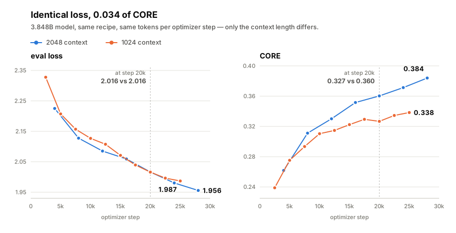
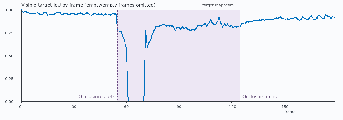
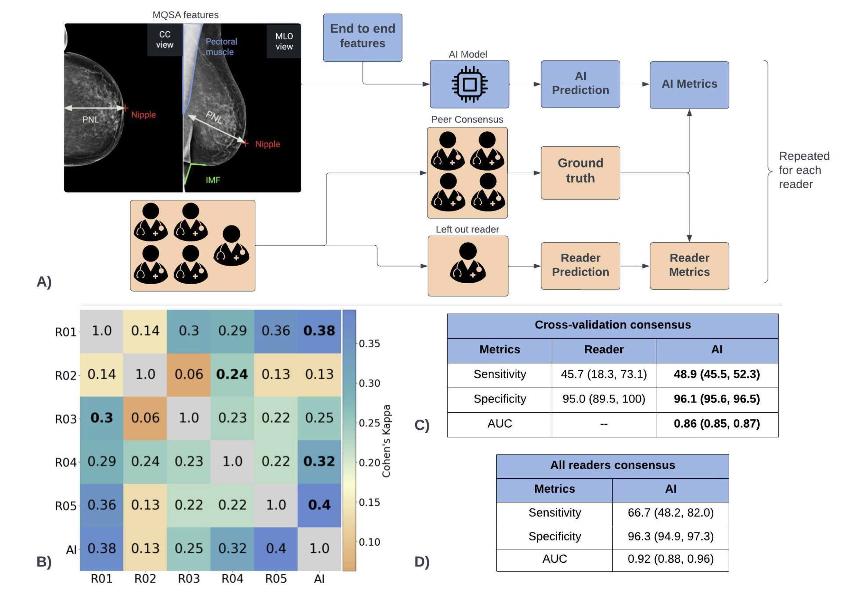
I wanted to see language and understanding emerge from random weights for myself, and to learn the parts you can only learn by starting from scratch. This project was written in the evenings, debugged on a 5090 and finished on rented B200s. It was heavily inspired by Andrej Karpathy’s nanochat.

The result is a 3.8B-parameter model scoring 0.384 on CORE, trained on 65B tokens in 43 hours for $998.

What follows is what worked, what didn’t, and what I still don’t know.

My model is larger than nanochat d32 and took similar wall-clock time. B200s were better value per unit of work than H100s. But for roughly the same money as nanochat’s $1,000 configuration, this lands meaningfully ahead of it. An encouraging data point about what’s reachable outside a lab or a mega company with millions in compute budget. As the frontier moves, $1,000 takes you further and further.

Setup

I’ve built little-lm as a config-driven framework for training small decoder-only LLMs. Every run is fully specified by a YAML file: model, dataset, optimizer, schedule, callbacks. Components self-register into a global registry and get resolved by name, so swapping an optimizer or a dataset is a one-line config change.

Good infrastructure pays for itself almost immediately. Ordinary software engineering discipline (Things like separation of concerns, clean interfaces, components you can swap in) matters a lot in AI work. It cost me a little at the start, and a couple more times afterward to fix bad contracts or suboptimalities. But this time investment pays for itself at the first convergence problem you encounter. I found that a great infra is the infra that almost never requires you to edit code manually. If you can read the config and understand exactly what happens, and there are no hidden mechanics, it means you have done a good job. The following report is the result of being able to express experiments as a three-line YAML diff rather than a branch.

The final model is Llama-style: RMSNorm, RoPE, GQA (24 query heads, 8 KV heads), relu² MLPs, QK-norm, logit softcap, per-layer learnable residual scalars, and ResFormer-style value embeddings.

Worth noting that the value embeddings are 19% of the parameter count. 14 tables of vocab × kv_dim, one on every other layer.

Results

Early experiments

Before good runs there were many bad ones.

I trained an 858M Llama on FineWeb-Edu for 16.4B tokens, 5.8 days on a single A100. AdamW at 2.5e-4, cosine decay to zero, 5% warmup, batch 256 via gradient accumulation, 2048 context.

The result: PIQA 60.45%. GPT-2 124M scores about 63%. I had spent six days of compute to build something worse than a model seven times smaller, from 2019. Generations were repetitive and borderline nonsensical.

The loss curve told the story.

1. Cosine decay to zero. The curve went completely flat after about 70% of the steps. The final 30% of the compute budget produced essentially nothing as the learning rate might be too low. Linear cooldown holds a useful rate much later.
2. Peak LR too conservative. 2.5e-4 is low for 858M parameters. You can be quite aggressive for those small models.
3. AdamW on everything. Muon should be meaningfully better per-token for the matrix parameters at this scale. In fact this was demonstrated pretty quickly in ablation runs.
4. The data. FineWeb-Edu is decent. It is not the best available.

Five changes came out of that post-mortem. Together they are the difference between the run above and a model that beats GPT-2 by a wide margin.

Trapezoidal LR schedule. Warmup for 5%. Hold flat and finish with linear cooldown over the last 50% to 5% of peak. The point is that the model keeps learning until the end instead of coasting through the tail. In the 3.8B run the eval loss was still descending at the final step, which is exactly the behavior the 858M run failed to produce.

Muon for matrix parameters, AdamW for everything else. Muon is slower per step (Newton-Schulz orthogonalization isn’t free, about 25% in a shallow-accumulation benchmark) but that cost is paid once per optimizer step: at 7 gradient-accumulation steps it dilutes to ~4%. Measured against total run time the convergence is much faster overall.

ClimbMix instead of FineWeb-Edu. This was a tremendous jump in convergence speed. Exactly as Karpathy found as well.

FP8 + vocab padding. FP8 training via torch._scaled_mm with dynamic tensorwise scaling on all three GEMMs, and padding the vocab from 50,257 to 50,304 (a multiple of 64) so the tensor cores are happy. Together, +33% throughput mostly from fp8.

1024 context instead of 2048. Halving the context roughly doubles the batch size at fixed memory. Throughput barely changes per token. We are still dominated by the MLPs which is a good sign we are using the hardware effectively. Below we will discuss the impact of the context length on the model.

Here is the whole run:

~480,000 tokens/sec in steady state, which puts 57.3B tokens at 33 hours. The wall clock was 35.9h. The difference is the CORE evaluations, which took about 15 minutes each (ten of them over the run) and consumed 7% of the total.

Re-running this identical recipe at 2048-token context scored 0.3840. Almost all of that gap turned out to be some tasks that were very context dependent.

On the GPUs themselves: 92% SM activity, 40% SM occupancy. High activity means the SMs almost never went idle. No dataloader starvation or network waits, which is the payoff for downloading the shards locally instead of streaming, which would leave us vulnerable to a small hugging face network hang. The low occupancy is what back-to-back large GEMMs look like: matmul kernels trade occupancy for register-tile size on purpose. Compute-bound and well fed, great signal we are using the hardware well and we can extend every dollar we spend into a better model.

That’s about 1,047 TFLOP/s sustained per B200, or ~25% MFU against Blackwell’s dense FP8 peak. (Against the bf16 peak it reads as 50%, which is the number that matters a bit more because not even all the linear layers run in FP8.)

The distributed strategy is plain old DistributedDataParallel. At 3.8B on a single node, gradient communication was never the constraint, and the sharded-optimizer machinery turned out to be unnecessary.

Increasing throughput

Renting GPUs isn’t cheap, at work you often think about the quality of the model before its cost. When it’s your own money burning, throughput matters a lot more all of a sudden.

This took real work on a single RTX 5090, before I ever rented a node. Baseline 858M model, bf16, compiled: 26,144 tok/s. Final: 37,621 tok/s.

FP8 (+25%). All three GEMMs (1 forward and 2 backwards) in FP8 with dynamic tensorwise scaling. Requires SM90+ but that is quite a nice throughput jump.

Vocab padding (+33% cumulative). Padding 50,257 → 50,304 costs 47 unused embedding rows and unlocks the fast tensor-core path. Nearly free.

Fused linear cross-entropy (+44% cumulative). Liger’s FusedLinearCrossEntropyLoss fuses the lm_head matmul into the loss and chunks internally, so the full (B*T, vocab) logits tensor is never materialized. Measured head-to-head at the same batch size it is 6% slower:

Even though it’s slower per step, it buys back a good amount of VRAM (8 GB on my 5090) so the increase in micro-batch size more than makes up for the lost 6%. Claude was quick to reject it because it was 6% lower, but overall it was a great way to claw some extra throughput.

Non-gated MLPs. Dropping the gate projection (SwiGLU → relu², two matmuls instead of three) on the small model: 183,035 → 214,173 tok/s and 6 GB less VRAM. One caveat from the ablations: a SwiGLU intermediate ratio of 2.75 does not transfer to relu². The model learns noticeably worse. Use 4× for non-gated.

bf16 master weights. Keeping the optimizer master weights in bf16 rather than fp32 cut VRAM 27% and raised throughput from 640K to 1.4M tok/s on the 1.5B config. That was a huge speed-up, 2.2×. The quality cost is real but small: CORE 0.22 vs 0.23 at 4,000 steps. When you’re optimizing for capability per dollar, careful dtype handling is one of the highest-leverage and underdiscussed knobs available.

Hardware. Same code, 150M model, FP8: RTX 5090 at 184,662 tok/s, B200 at 477,440 tok/s. 2.59× from hardware alone, before accounting for the extra VRAM letting you push batch size further.

What didn’t work

Document-boundary masking with flex attention. Packing documents into one sequence lets tokens attend across boundaries, so I fixed it properly: per-token document IDs and mask out attention so each token can only attend to its current document. It was elegant, but I deleted all of it. Andrej Karpathy also found that cross-document leakage does not make things much worse under BOS-aligned packing. Best-fit packing replaced it in ~10 lines, and attention went back to an unconditional F.scaled_dot_product_attention(..., is_causal=True). I believe this is also conditional on the dataset and the training documents.

Liger RMSNorm and RoPE. RoPE was 2.2× faster in a microbenchmark and produced no measurable change in end-to-end throughput. RoPE is not part of the critical compute bottleneck at this scale. RMSNorm was outright slower than PyTorch 2.9’s built-in F.rms_norm (0.41ms vs 0.25ms). Both reverted, not worth the complexity.

Nanochat-style initialization. Embeddings at N(0, 0.8), linear weights uniform, output projections zero-initialized so the residual stream starts as pure identity, LM head at N(0, 0.001). Theoretically much nicer than GPT-2’s N(0, 0.02) everywhere. The loss curve starts marginally lower and the two curves overlap by ~1,500 steps. No measurable quality difference. I kept it, but for aesthetics, not evidence.

Streaming datasets. Great for getting started, wrong for a real run. Even when the network looks healthy, local shards gave 2-3% more throughput, and occasional network dips cost far more than that. For runs longer than a few hours, it’s worth it to pay the download once at the start of training.

Ablation on value-embedding

Value embeddings were 721M parameters for a 3.8B model. I trained the same model with the same config with value_embeddings: false and compared it against the original run, which I’d already paid for, out to 12,500 steps and 29B tokens.

0.46% better loss and 3.2% better CORE, for 19% more parameters. The throughput is identical, because value embeddings are lookups. They cost memory and optimizer state but essentially no FLOPs.

Two interesting findings:

• Value embeddings bought the equivalent of about 1,200 training steps. Here is how to price that: between steps 10,000 and 12,500 my baseline loss fell 0.0194, so 2,500 steps buys roughly that much. The value-embedding advantage is 0.0096, about half of it — call it 1,200 steps out of 25,000. So 19% more parameters is worth ~5% more training.
• CORE moved about seven times more than loss did (3.2% vs 0.46%), and the gap shrank steadily during training. That’s worth knowing if you’re using CORE to make decisions: it’s an accuracy metric, so items near the decision boundary flip on tiny logit changes, and it’s centered against a random baseline, which amplifies relative differences while scores are still low.

Value embeddings are useful for a small model and come at almost no throughput cost. Spending a little bit of VRAM on this gives the model a form of bias toward certain concepts that might be useful for CORE.

Discussion

Misleading micro-benchmarks

We could be tempted to believe that 1024 tokens context is plenty for a high CORE score. Going back through the per-task logs, that conclusion is wrong on some tasks that are very context sensitive.

3 of the 22 CORE tasks have prompts that essentially never fit in 1024 tokens:

SQuAD is the striking one. It doesn’t stagnate, it decays monotonically to exactly zero: 0.1478 → 0.0617 → 0.0099 → 0.0007 → 0.0000. The model gets steadily worse at this task the longer it trains, which is not a thing models normally do.

Two details explain it. SQuAD is a 10-shot task in the DCLM bundle, so each prompt is ten worked examples followed by the real one. Median of 1,998 tokens on my eval data. Not one fits in 1024. And when a prompt is too long my harness keeps the last max_seq_len tokens.

The test passage sits at the end, so it always survived; a test example is only ~169 tokens. What got truncated was the ten demonstrations. The model was reading the passage and the question, and almost never seeing the examples that teach it the expected output format. Since SQuAD is scored on exact-token match against the gold answer, fluent prose scores zero every time.

That also explains the decline. An early, high-entropy model occasionally emits something short and generic that happens to match. As it sharpens it commits to well-formed continuations, and the accidental hits disappear. Funnily enough, getting better at language made it worse at guessing right by accident.

boolq shows a gentler version of the same shape. It peaks at step 10,000 (0.6294) and declines to 0.5131. Language identification never moves off chance at all.

In short, 0.338 was measured with three of 22 tasks scoring near-zero for reasons that have nothing to do with model quality, just the size of the context length being fed to it.

The effect of larger context

As we have seen, if we want the highest CORE score possible we need larger context. But this has consequences on the training throughput.

Double the context length, halve micro-batch to hold VRAM constant, so tokens per optimizer step stayed identical. I stopped it at ~28,000 steps to save the last few hours of rental, so the learning-rate warmdown never fully completed and the number below is a lower bound.

CORE went from 0.3384 to 0.3840.

At step 20,000 the two runs have the same eval loss to four decimal places (2.0160 vs 2.0164) and differ by 0.034 on CORE. It was surprising to see that low level of correlation between CORE and eval loss on the ClimbMix dataset.

squad and boolq alone are 83% of the gain. boolq contributes the most, because its random baseline is 0.5 and CORE centers against that: a raw +0.196 becomes a centered +0.517. Strip those two and the remaining twenty move +0.008 in total, roughly what 14% more tokens buys on its own.

Language identification went from 99.7% cropped to 14% cropped and moved +0.005. This is by far the hardest task in the CORE evaluation benchmark for our current model.

A couple of tasks got worse: commonsense_qa dropped 0.072, cs_algorithms 0.031. Across 22 tasks some movement in both directions is expected.

2048 was worth paying for as a measurement decision, not a quality one. It cost 9% throughput (480K → 437K tok/s), and outside the tasks that couldn’t be scored at 1024 it bought almost nothing. 1024 is fine for training and a “cheap” way of getting your model to a good CORE score. 2048 unlocks some tasks that are very context bound.

Future work

Limitations

Four things I never ablated. Peak LR, from nanochat’s sqrt(768/d_model). I didn’t really want to spend money to sweep learning rates. I moved from cosine to trapezoidal because of the 858M post-mortem, there could be schedules out there that are more efficient. QK-norm, on by default and never toggled off. And the GQA ratio, since it’s a nice lever to save on memory.

Most of those are inherited from nanochat rather than tested here. That is a defensible way to spend a small budget — someone else already paid for the experiment — but it means I am trusting that Karpathy’s results transfer to my model, data and scale.

Open questions

There is a lot of interesting work I’d want to pursue if I had more time and resources:

• Value embeddings versus reallocation. The comparison above was VE against nothing. The one that matters is VE against spending those 721M on something else.
• 1024 versus 2048 at matched wall-clock. The rerun changed context and ran longer, so it settles the measurement question but not the quality one.
• Why commonsense_qa regressed by 0.072 at the longer context, when nothing about that task involves long prompts.
• Sharding the optimizer, the way nanochat does. I used plain DDP with a single-GPU Muon, which means every rank holds a full copy of the optimizer state and redundantly recomputes the same Newton-Schulz update. nanochat drops the DDP wrapper entirely and does ZeRO-2 sharding inside the optimizer, overlapping reduce-scatter, compute and all-gather. The memory win is the certain one, and freed memory turns into batch size, which is tokens for the same dollars. Whether the redundant orthogonalization also goes away depends on how the sharding is done: Muon needs the full gradient matrix, so splitting a matrix across ranks doesn’t help, while giving each rank whole matrices of its own would. I haven’t explored that at all but I think it would be a great way to further increase the total training throughput at the cost of some extra machinery.
• Additional data exploration. I haven’t had a lot of time for data analysis on either the CORE benchmark or the ClimbMix dataset. I’m sure this would help us claw even higher performance with the same compute budget.

Closing thought

GPT-2 was a frontier result in 2019, produced by a well-funded lab with a large team, and its 1.5B model scores 0.2565 on CORE. 7 years later I beat that by a wide margin in my evenings, for $998, on hardware I rented by the hour.

The frontier moved, and everything came with it. Work that needed a lab can now be done by a single engineer in the evenings. I wonder what kind of insane machine we will be able to build in 7 years from now!

Appendix: the config

The whole run, flattened from the YAML includes into one block.

model:
  hidden_size: 3072
  intermediate_size: 12288      # 4x, non-gated
  num_hidden_layers: 28
  num_attention_heads: 24
  num_key_value_heads: 8        # 3:1 GQA
  head_dim: 128
  hidden_act: relu2
  gated_mlp: false
  qk_norm: true
  logit_softcap: 15.0
  layer_scale: true
  value_embeddings: true        # 14 tables, alternating layers
  tie_word_embeddings: false
  rope_theta: 10000.0
  rms_norm_eps: 1.0e-6
  vocab_pad_to: 64              # 50257 -> 50304
  max_position_embeddings: 2048
  dtype: bf16

engine:
  compile: true
  fp8: true
  precision: bf16
  total_batch_size: 2293760     # 20 x 2048 x 7 grad_accum x 8 GPUs
  loss: LigerFusedLinearCrossEntropyLoss(softcap=15.0)

optimizer:                      # composite, one group per parameter class
  matrix:        Muon   lr=0.02      momentum=0.95  wd=0.0
  embeddings:    AdamW  lr=0.1414    betas=(0.8, 0.995)  eps=1e-10  wd=0.001
  lm_head:       AdamW  lr=0.002828  betas=(0.8, 0.96)   eps=1e-10  wd=0.01
  value_embeds:  AdamW  lr=0.0707    betas=(0.8, 0.995)  eps=1e-10  wd=0.01
  scalars:       AdamW  lr=0.005     betas=(0.8, 0.95)   eps=1e-10  wd=0.05

scheduler:
  trapezoidal:
    warmup_ratio: 0.05
    warmdown_ratio: 0.50
    final_lr_frac: 0.05

data:
  dataset: nvidia/Nemotron-ClimbMix  (karpathy/climbmix-400b-shuffle shards)
  tokenizer: gpt2 (tiktoken)
  block_size: 2048
  packing: best-fit, BOS-aligned
  batch_size: 20 per rank
  num_workers: 11

trainer:
  max_steps: 32000              # stopped at ~28,000 -> 65.3B tokens
  eval_every: 4000              # must divide max_steps or the final CORE is skipped

The AdamW learning rates follow nanochat’s sqrt(768/d_model) scaling rule; the Muon LR of 0.02 is inherited from there too.

Appendix: example text generation

The capital of France is Paris. It is the largest city in France and the second largest city in Europe
The french revolution happened in 1789 and 1799, and was a time of great change in france
At the center of the milky way there is a supermassive black hole. It is called Sagittarius A* (pronounced
Electrons orbit around the nucleus of an atom in a series of energy levels. The energy levels are numbered
Newton discovered the laws of motion and gravity. He also discovered the law of universal gravitation. Newton's

Unlike an object detector, it does not discover the target from a category prompt. It receives an initial segmentation mask that identifies the object of interest, then propagates that object identity through the rest of the video.

The underlying idea is broader than segmentation: preserve a compact, searchable representation of earlier observations so that information can be recovered over long sequences.

I wanted to understand what this memory mechanism costs, what the initial mask actually does, and how the model behaves when the target is occluded. I built a small synthetic sequence, ran XMem on my RTX 5090, counted FLOPs across its inference phases, and recorded the IoU before and after occlusion.

The main results were:

• XMem propagated a first-frame target mask without fine-tuning on the synthetic video.
• It preserved target identity in the presence of a similar-looking distractor.
• Its predicted mask disappeared under full occlusion and recovered as the target became visible again. It didn’t confound the occluded object with the similar looking one still visible.
• At 480 short-side resolution, it processed the 180-frame sequence at ~64 FPS using ~940 MiB of peak CUDA allocation with AMP on my 5090.
• At 720 short-side resolution, throughput fell to ~42 FPS and peak allocation increased to ~2500 MiB.
• At 480p, mean visible-target IoU was 0.864; the prediction was correctly empty for all six fully occluded frames.
• The segmentation decoder, not the memory read alone, dominated propagation FLOPs.

The task is mask propagation, not object detection

XMem solves semi-supervised video object segmentation. For one object, its initial inputs are conceptually:

RGB frame:    [3, H, W]
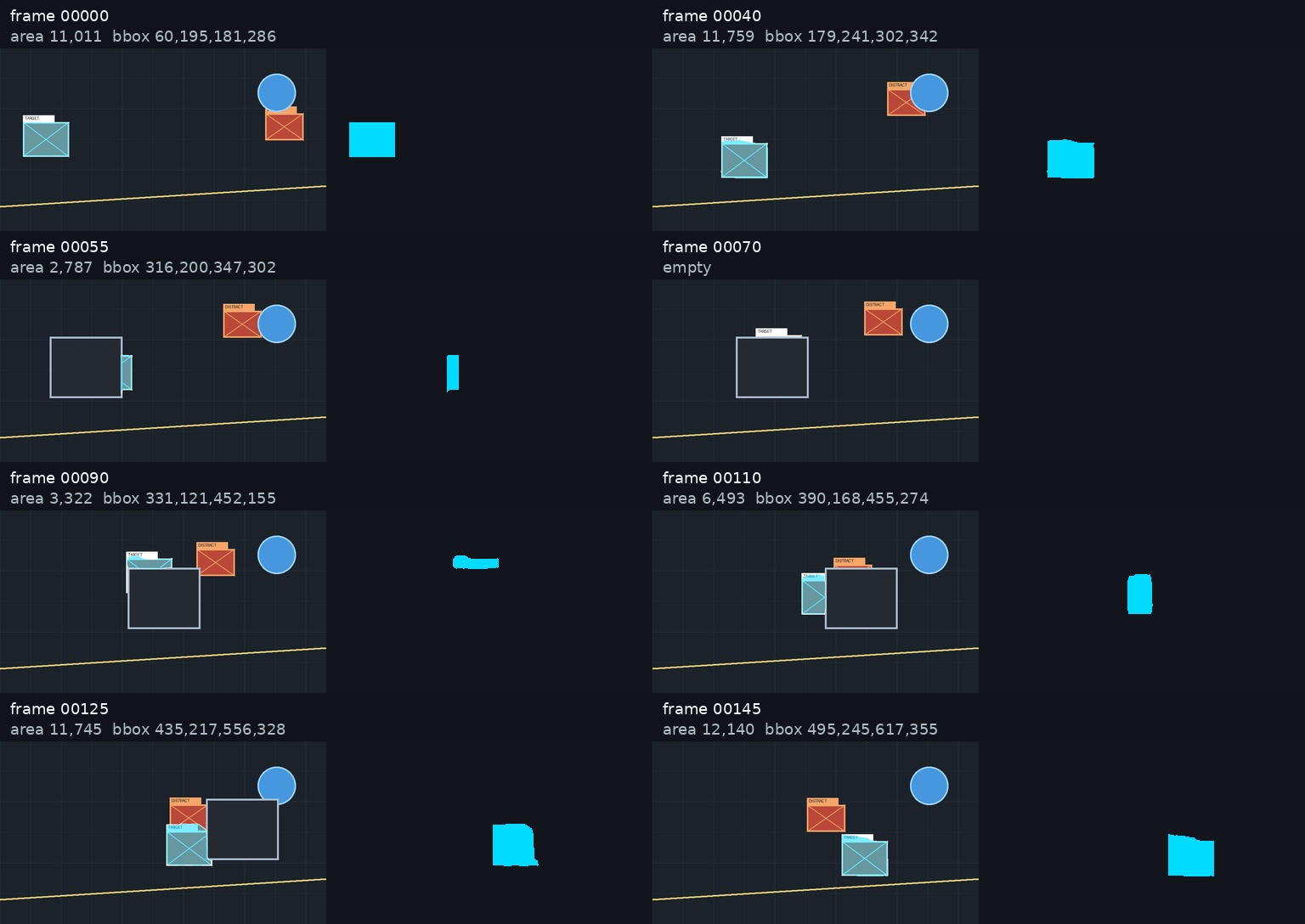
object mask:  [1, H, W]

The mask answers a question that RGB alone cannot answer: which object should the model follow? This matters when a frame contains multiple plausible targets. The model does not need a semantic label such as “car” or “person,” but it does need a seed that establishes object identity.

The frame is encoded into spatial features. XMem creates compact keys for matching and richer, mask-conditioned values for object information. At a high level:

initial frame + mask -> object-specific key/value memory
current frame        -> query keys
memory match         -> retrieved object features
retrieved features   -> current-frame mask

The synthetic frames are generated at 864x480. Both dimensions are divisible by 16, the stride-16 feature grid is 54x30, or 1,620 positions. With the released checkpoint, a simplified single-object memory entry has shapes similar to:

key:    [1, 64, 30, 54]
value:  [1, 1, 512, 30, 54]

The key is shared matching information. The value includes an object dimension because it carries information conditioned by the input mask. This distinction is the core of the model: use a relatively small representation to find relevant memories, then retrieve a larger representation containing target-specific detail.

A synthetic occlusion test

The synthetic sequence includes three elements:

• a masked target moving through the frame;
• a similar red distractor following a different trajectory;
• an opaque foreground occluder that fully covers the target during part of the sequence.

Only the first-frame target mask is placed in XMem’s Annotations input. XMem must propagate that initial identity through all later frames without correction. A separate EvaluationMasks directory contains the visible target mask for every frame. These evaluation masks subtract the opaque occluder and are never passed to the model. A second evaluation-only mask tracks the visible distractor.

The following contact sheet samples the sequence before, during, and after occlusion. Each sample contains two panels. The left panel is the RGB frame with XMem’s prediction overlaid in cyan. The right panel isolates the predicted foreground mask. The reported area is the number of predicted foreground pixels, while the bounding box gives the prediction’s extent in the original frame coordinates.

This makes the failure and recovery sequence visible rather than reducing it to one aggregate metric:

• Before occlusion, XMem followed the seeded target.
• As the occluder covered the target, the predicted foreground area shrank.
• Under full occlusion, the prediction became empty.
• As the target reappeared, XMem first recovered partial masks and then returned to the target.
• It did not visibly switch identity to the similar distractor in the sampled frames.

This is not evidence that XMem predicts an object’s hidden extent. It did not produce an amodal mask behind the occluder. The result is better understood as visible-region segmentation with identity recovery after reappearance.

The per-frame masks turn this into a quantitative test. IoU is computed against the visible target rather than its hidden full extent. Empty-vs-empty IoU is undefined, so the six fully occluded frames are excluded from mean IoU and reported separately. XMem produced an empty prediction on all six. On the remaining frames, the 480p AMP run achieved:

The target first reappeared at frame 69 and crossed IoU 0.5 at frame 71, a recovery delay of two frames. On average, 0.85% of predicted pixels overlapped the distractor; the maximum on any frame was 12.90%. The partial-occlusion and after-reappearance slices are intentionally not disjoint: the target is still partially covered for some frames after it first reappears.

The timeline exposes behavior that the aggregate means hide. The shaded interval and dashed boundaries mark the start and end of occlusion, while the orange line marks the target’s reappearance. Missing points correspond to the six empty-ground-truth frames, where IoU is undefined; those frames are covered by the separate correct-empty result rather than being assigned an IoU of 1.

Inference cost depends on the frame type

XMem does not perform exactly the same work on every frame. I counted operations for three phases at 864x480 with one object:

The first annotated frame initializes object memory and is the least expensive of these phases. A normal propagation frame reads memory and decodes a segmentation. A memory-update frame encodes a new value to write back into memory, adding about 86.25 GFLOPs.

The ValueEncoder accounted for about 88.86 GFLOPs in the module table, which closely matches the measured increase. This makes the tradeoff behind XMem’s memory-update interval concrete: writing more often gives the model fresher object information, but value encoding is not free.

The decoder dominates propagation compute

I initially expected content-addressed memory matching to dominate inference. At this resolution, it did not. The propagation breakdown was:

Most decoder cost came from higher-resolution fusion and upsampling:

This changes how I would reuse XMem’s ideas in a smaller system. The key/value memory pattern is attractive, but copying the full segmentation decoder and mask-conditioned value encoder would bring most of the compute with it.

Resolution is the practical constraint

The wall-clock benchmark used the same 180-frame synthetic sequence:

Moving from a 480 to 720 short side increases pixel count by 2.25x. Throughput decreased by about 36%, while measured peak allocation increased by 2.65x.

The memory increase is not only caused by larger CNN feature maps. XMem compares current-frame query positions against stored memory positions. In this implementation, the dense similarity tensor is constructed before top-k selection. Increasing resolution therefore expands both sides of the matching operation: there are more locations in each stored frame and more query locations in the current frame.

An experiment above 720 short side made the workstation unresponsive, so I removed that case from the benchmark. This is not a universal resolution limit for XMem. It is a practical limit for this sequence, configuration, and workstation. Memory cadence, working-memory size, video length, object count, and software versions can all change the outcome.

One other result was counterintuitive: FP32 was faster than AMP at 480p, although it used more memory. On this run, FP32 delivered 74.59 FPS versus 63.87 FPS with AMP. Autocast overhead, kernel selection, TF32 behavior, and run-to-run variance could all contribute. I would not generalize from one run; repeated warmed-up measurements are needed before concluding that FP32 is consistently faster.

Closing thoughts

XMem is a useful example of explicit memory applied to video. Its first-frame mask creates object-specific memory, its compact keys support content-based lookup, and its values preserve richer information for mask decoding. On my synthetic test, this was enough to maintain identity through an occlusion and reappearance event without fine-tuning on the sequence.

The implementation is not lightweight. At 480p, a normal propagation frame required about 295 GFLOPs, and the decoder accounted for most of that cost. Memory-update frames were more expensive because value encoding added roughly 86 GFLOPs. Increasing resolution also produced a sharp memory increase because spatial memory matching grows with both stored and current-frame positions.

XMem’s most reusable idea is not necessarily its complete architecture. It is the separation between a small key used to find relevant history and a larger, object-conditioned value used to reconstruct detail. That pattern is applicable beyond segmentation, provided the memory lookup and decoder are designed around the resolution and hardware constraints of the final system.

fork: https://github.com/hugovergnes/XMem/tree/experiment/synthetic-occlusion-benchmark

But the same inductive biases inherently limit their flexibility when compared to vision transformers. ViTs, by treating images as sequences of patches, discard these biases in favor of learning global relationships directly from data. This flexibility has enabled vision transformers to excel in scenarios where vast amounts of labeled or pre-training data are available, leveraging their capacity to model long-range dependencies across the image. However, this does not work as well in medical imaging, where the available data is more limited and often has a very high resolution.

In this post, I’ll discuss my experience working with all those networks. How modern CNNs like ConvNext have evolved to remain relevant, how vision transformers such as Swin-V2 and PvT-V2 integrate hierarchical design principles to balance efficiency and expressivity, and how models like Hiera push the boundaries of self-supervised learning.

Locality assumes meaningful patterns or features can be found within small, localized regions of the input data. This concept is fundamental to how convolutional layers operate and why CNNs are so effective for spatially structured data like images. In practice, this is found in the size of the convolution kernels (33 or 55). As the filter slides through the image, only the pixels in the receptive field are considered.

In breast cancer, tumors often have a spiculated appearance. This star-shaped structure can be detected with this type of operation.

Translation equivariance means that when an input is translated (shifted) spatially, the feature map produced by the convolutional layer shifts by the same amount, preserving the spatial relationships. In other words the two operations commute:

This is useful in the medical field. When you want to find a tumor in a large image (like a medical scan), the precise location of the tumor does not matter that much. If it’s translated to the right or left, it should produce the same feature map.

This assumes that complex patterns can be built hierarchically from simpler patterns (e.g., edges → textures → objects). In a way, locality is the fine-grained detection of edges in the image, and spatial hierarchy allows the reconstruction of more complex structures. In ImageNet, you would typically detect edges, then a dog’s ear, and then a dog. This was initially how it was presented with AlexNet.

This assumes that the same feature can occur across different parts of the input, so the same set of weights (filters) can be used everywhere.

Once again, in our cancer detection example, this is adequate. Cancer can appear in different parts of scans; its low-level features (edges, etc.) should be detected the same way.

Transformers were initially proposed as an NLP algorithm, where each word was treated as a token. In computer vision, you need to divide images into patches and treat those patches as tokens. Unlike CNNs, Vision Transformers do not rely on locality as an inductive bias. Instead, ViTs treat the input image as a sequence of patches, much like words in a sentence for natural language processing. This approach allows ViTs to learn global relationships between image regions from the start, without assuming that important features are localized.

This is both a curse and a blessing for Transformers. It’s a curse because the attention operation scales quadratically with the size of the image or as you reduce the size of the patches. An alternative is to use bigger patches for bigger images, but that limits the effective resolution of the patches processed in the transformer. This usually leads to poor performance. But this can also be a blessing because, if you can afford it, you can relax the inductive biases and generally get better performance.

ConvNext reimagines traditional CNNs with a modern twist, incorporating design elements inspired by vision transformers, such as large kernel sizes, depthwise convolutions, and layer normalization. While retaining the strong inductive biases of CNNs, ConvNext reduces these limitations by improving flexibility and scalability. This makes it highly competitive on benchmarks, offering a well-regularized alternative to transformers, especially in data-limited settings.

NFNets (Normalizer-Free Networks) are convolutional neural networks introduced by Google Research in 2021, and they share similarities with modern CNNs like ConvNeXt in their architectural improvements. Most notably, they remove the use of Batch Normalization (which has several problems of its own). They also incorporate several design features found in ConvNeXt, such as depthwise separable convolutions for efficiency. This operation splits the standard convolution into two steps. First, a depthwise convolution applies a single filter per input channel rather than aggregating across all channels. Second, a pointwise convolution aggregates depthwise information across all channels. It also proposes better initialization, optimization methods, etc.

Overall, scaling those models results in performance as good as that of Vision Transformers.

Similarly, Vision Transformers have undergone considerable modernization in the last couple of years.

Most noteworthy, and distilled in many variants, is the addition of a hierarchical structure to the network. This drastically reduces the computational cost of those networks. Swin-V2 introduces shifted windows, which enable hierarchical feature learning while maintaining global context through cross-window connections. This mechanism avoids redundant computations by focusing on non-overlapping regions of the input, significantly reducing complexity compared to traditional attention mechanisms.

On the other hand, PvT-V2 achieves a hierarchical structure by progressively reducing spatial dimensions through patch-merging layers, allowing the model to capture multi-scale features efficiently. These hierarchical designs not only improve scalability but also enhance performance on tasks requiring both fine-grained details and global understanding, making them highly effective for large-scale vision applications. In my work, I found PvT-V2 to be an outstanding model, offering high accuracy with an unusually small number of parameters and low computational cost. For example, at a similar performance level, PvT-V2 would take half the memory of ConvNeXt and train twice as fast.

Let’s mention something that is becoming ubiquitous in Transformers: Flash Attention. This is now a default setting in PyTorch if the hardware can support it. Flash Attention is an optimized attention mechanism designed to reduce memory usage and computational overhead, particularly for large models. Unlike traditional attention mechanisms, which have quadratic memory complexity with respect to the sequence length, Flash Attention leverages efficient memory access patterns and kernel optimizations to compute attention in a memory-efficient way. By implementing a more compact representation of the attention matrix and using hardware acceleration techniques, Flash Attention can handle longer sequences with significantly lower memory consumption and faster processing speeds, making it ideal for tasks with large-scale inputs, such as transformers applied to vision and language models. This makes it a promising technique for scaling up models without compromising performance.

• A lot of discussion revolves around how transformers work. There is an overall impression (which I share) that transformers learn more texture-based than shape-based features when compared with CNNs. This is due to the inductive biases we just mentioned.
• ViTs excel in tasks where global context or relationships are crucial, especially when sufficient data and computational resources are available. CNNs are more efficient and effective when local patterns dominate the task (e.g., detecting edges or textures) or when computational resources are limited.

With ChatGPT, SAM2, and more AI-powered solutions, I’ve noticed a shift toward making these models more readily available to end users. This is a welcome change, but it comes with challenges in making the demo compelling. This takes more engineering effort than research effort. I predict that this trend will consolidate and that we will see more applications that leverage the low latency of modern hardware.

I also suspect that self-supervision will become more prevalent, especially for tackling scenarios where data is not available. In the medical field, this could involve a new scanner type. If you have trained an AI algorithm, you would like it to also work well on newer, more sophisticated versions of the scanner. But of course, since it is newer, you don’t have as much training data available. Pre-training can help level that field.

Finally, as much as I would like to see a change in paradigm, it looks like a moonshot. I think the sequence-to-sequence approach in ViT is ill-suited for vision, but it clearly yields remarkable performance.

Purpose

Safeguards are needed to protect autonomous artificial intelligence (AI) rule-out systems for breast cancer screening from exams with image quality (IQ) deficiencies that could impair the sensitivity of the models. This work introduces an AI system that assesses IQ in full-field digital mammography (FFDM) exams and evaluates it against expert radiologists.

Materials and Methods

An AI system was trained to identify screening FFDM exams that require a technical recall due to inadequate IQ. The system evaluates positioning and blur, with features based on MQSA criteria as well as learned features. This model was evaluated on 1,100 screening exams from 2 independent held-out U.S. datasets (Dataset 1: 835 exams, from 2012-2019; Dataset 2: 265 exams, from 2002-2009) that were labeled as requiring recall or not by 5 breast fellowship-trained radiologists with at least 15 years of experience (used for testing only).

The performance of the model was first evaluated based on a reference standard of the median assessment of the 5 readers. To compare the AI and individual readers, we employ an evaluation methodology similar to leave-one-out cross-validation. In this method, we left out one reader at a time to establish a consensus based on the assessments of the other readers. Then, we compared the excluded reader and the AI model to this consensus. We repeated this for each reader to ensure an unbiased comparison between the AI and readers.

Results

The percentage of exams recalled (inadequate IQ) by the 5 readers ranged from 0.7% to 13.7% (Mean: 6.4% Standard Deviation: 4.8%). Pairwise agreement between the readers was low (Cohen’s kappa: 0.06-0.36). Based on a reference standard established by all 5 readers, the AI model achieved a sensitivity of 66.7% [48.2%, 82.0%], a specificity of 96.3% [94.9%, 97.3%], and an area under the receiver operating characteristic curve (AUC) of 0.92 [0.88, 0.96]. The sensitivity of the model increased when more readers labeled a sample as inadequate (3/5 readers: 56.5%, 13/23; 4/5 readers: 83.3%, 5/6; 5/5 readers: 100.0%, 4/4). Based on the cross-validation approach, the system exhibited comparable performance to the mean of the readers in sensitivity (AI: 48.9% [45.5%, 52.3%]; Mean Rad.: 45.7% [18.3%, 73.1%]) and specificity (AI: 96.1% [95.6%, 96.5%]; Mean Rad.: 95.0% [89.5%, 100.0%]). The system achieved an average AUC of 0.86 [0.85, 0.87].

Conclusions

This study demonstrates that an AI model can achieve comparable performance to expert radiologists in assessing IQ for mammography, overcoming the inherent challenges in the task’s subjectivity.

Clinical Relevance/Application

AI systems that provide an automatic check on IQ can assist with improving image acquisition and also help safeguard cancer-detecting AI models from exams with poor IQ.

The Challenges of ViT with high-resolution images

As the resolution of images increases, the computational and memory demands of ViTs become increasingly prohibitive. Because the number of tokens grows quadratically with the image resolution! This quickly becomes prohibitive. This is where Hierarchical Vision Transformers (Hiera) shine as a more efficient and scalable alternative.

Vision Transformers rely on dividing an image into fixed-size non-overlapping patches, which are then treated as tokens for the model. The key issue arises from the fact that each token is processed through all stages of the transformer. As a result, when working with high-resolution images, the number of tokens increases dramatically, leading to a massive increase in computational complexity and memory usage. This makes ViT less feasible for large images, where processing all tokens at every stage becomes impractical.

How Hiera addresses these issues

Hiera, on the other hand, takes a hierarchical approach to token processing. Pooling the query tokens (Q) significantly improves efficiency. Unlike ViT, Hiera does not process all tokens at every stage. Instead, it selectively reduces the number of tokens passed through deeper layers. This hierarchical tokenization ensures that only the most relevant tokens are processed at higher levels, drastically reducing the memory footprint while maintaining or even improving model performance.

In high-resolution image tasks, this approach allows Hiera to maintain a more manageable number of tokens at each stage. By focusing on the most important information at each level, Hiera can capture fine-grained details without the need to process the entire set of tokens throughout the model. This makes Hiera a strong candidate for replacing ViT, especially when working with images of very high resolution.

Further development for higher resolution images

However, many groups, including mine at work, witnessed something unexpected. Hiera really doesn’t generalize well to different resolutions. This shouldn’t happen: the only component of a Vision Transformer that requires knowledge of the input resolution is the positional embedding. There is no reason for this to cause any problems for the higher-resolution downstream task. It turns out the problem arose from an interaction between Window Attention and the positional embedding. Hiera was then used in the trunk of the image encoder for SAM2. It was one of the key contributions that enabled the creation of this compelling real-time demo.

This was an exciting innovation to see, as it led to great improvements. In a field where we need more players, we need more papers that make it possible for smaller groups to propose SOTA systems with fewer resources.

In my experience. Pre-training, training and inference.

Hiera holds much promise as it addresses the prohibitive memory usage of non-hierarchical Vision Transformers. However, they still rely on a sequence-to-sequence paradigm that is not ideal for vision. In my experience, it appears that the inductive biases inherent to CNNs make for better models. Typically, ConvNeXt is a very hard model to beat in downstream prediction tasks.

In my experience, Hiera undeniably beats ViT. But it is still underwhelming in many aspects. First, the MAE pre-training step is computationally expensive. This is a heavy constraint on relatively GPU-poor groups. Second, the performance of the fine-tuning step is lackluster. Not only does it still require a decent amount of data for the prediction task, but the model also struggles to compete with its more advanced counterparts (ConvNeXt, PvT, MViT, Swin-V2) that are initialized from ImageNet and trained directly on the task (with no specific pre-training task). I haven’t managed to make it really competitive despite my best efforts and extensive experimentation (different masking ratios, layer-wise learning rate decay, high batch sizes, and many different fine-tuning settings). It gets better if you keep the earlier layers unchanged (prefer downsampling the image over cropping, keep the patch size fixed between pre-training and fine-tuning, etc.), but it never becomes SOTA on the proprietary datasets I worked on. Third, it looks like Hiera has some convergence issues. The pre-training step might result in occasional crashes where the loss suddenly becomes NaN and all the weights are messed up. All of this is for a speed increase in the forward and backward passes that is marginal for relatively high-resolution images (~3000 × 2000).

Closing thoughts

I think Hiera and MAE in general are interesting approaches. But they offer little utility when you try to apply them without some of the biggest datasets out there, coupled with serious GPU power. Nonetheless, I think pretext tasks for pre-training make sense and might help in many downstream scenarios. I’m excited to read more research on this topic.

In this repository, we approach it in a simpler manner where we solve each sudoku as a human would, by putting a digit down only if no other digits can go in this cell or if that digit can only go here.

The code involves representing the Sudoku board as a Table class, where each individual cell is an instance of the Cell class. I did this project as a way to make a long flight interesting, so the goal was to have fun with a puzzle that has fascinated me since I was a kid while applying and practicing principles of good software engineering.

The whole code revolves around a Cell class representing a cell in the Sudoku board. Once you have this, you just need to keep track of candidate values, and it solves itself!

class Cell:
    def __init__(self, pos, value=0):
        """_summary_

        Args:
            pos (Tuple): Position of the Cell in the sudoku table.
            value (int, optional): Value in the cell. Defaults to 0 if the cell is unknown.
            candidate_values (set): Possible values in that cell. If the cell is already set to
            non-0. Then It is empty.

        Raises:
            RuntimeError: _description_
        """
        self.pos = pos
        self.value = int(value)
        self.candidate_values = set()

    def __str__(self):
        return str(self.value)

    def __eq__(self, other):
        if isinstance(other, int):
            return self.value == other
        return self.value == other.value and self.value == other.value

    def is_known(self):
        return self.value is not None

    def get_value(self):
        return self.value

    def set_value(self, value):
        self.value = value
        self.candidate_values = set()

    def get_candidate_values(self):
        return self.candidate_values

    def get_prohibited_values(self):
        prohibited_values = sorted(
            set([i for i in range(1, 10)]) - self.candidate_values
        )
        return prohibited_values

If you liked this post, you should check out my repo.

The implementation was designed to be lightweight and adaptable. While I initially ran the training on a CPU, the model can easily be transferred to a GPU using Google Colab for faster results. If you’re interested in experimenting with it, I’ve also included a ready-to-go Colab notebook that automates the setup. Special thanks to the authors of the original paper on Path Integral-based GNNs and the guidance from CS224W.